1D-RISM Tutorial

In RISM calculations with Quantum ESPRESSO, 1D-RISM first gives the correlations among the solvent species (the structure of the solution itself), and 3D-RISM or ESM-RISM (Laue-RISM) then uses them to obtain the solvent distribution around the solute. This page takes the 1D-RISM part, which runs first, out of the "H₂O in NaCl(aq)" calculation of the example PW/examples/RISM_example. For the theory, see 1D-RISM.

Setup

RISM is switched on by trism = .true. in &control; the solvent is specified with the &rism namelist and the SOLVENTS card. The parts relevant to 1D-RISM are:

 &control
    calculation = 'scf'
    trism       = .true.
 /
 &rism
    nsolv    = 3            ! number of solvent species
    closure  = 'kh'         ! closure equation (Kovalenko-Hirata)
    tempv    = 300.0        ! temperature (K)
    ecutsolv = 144.0        ! cutoff for the solvent (Ry)
    ! 1D-RISM's setting
    starting1d      = 'zero'
    rism1d_conv_thr = 1.0e-8
    rism1d_maxstep  = 10000
    mdiis1d_size    = 20
    mdiis1d_step    = 0.5
 /
SOLVENTS {mol/L}
 H2O  -1.0  H2O.spc.MOL
 Na+   0.5  Na+.aq.MOL
 Cl-   0.5  Cl-.aq.MOL

• Each line of SOLVENTS gives the solvent name, its concentration and its MOL file. A negative concentration means the density written in the MOL file is used (1 g/cm³ for water). Here Na⁺ and Cl⁻ are 0.5 mol/L each, i.e. 0.5 M NaCl(aq).
• A MOL file gives the structure and the classical force field (charge and Lennard-Jones parameters of each atom) of a solvent molecule. Water is the SPC model (with modified LJ parameters for hydrogen). The files are in the example's MOL/ directory and are read from pseudo_dir.

Run the example as follows. The calculation takes a few tens of seconds.

cd q-e/PW/examples/RISM_example
./run_example_3D-RISM

The total energies shown here agree with the reference outputs distributed with the example within \(10^{-6}\) Ry.

How 1D-RISM proceeds

The beginning of the output shows the 1D-RISM settings and its convergence.

     1D-RISM info
     ------------
     closure equation        =           KH
     temperature             =     300.0000  kelvin
     coulomb smearing radius =       2.0000  bohr
     number of solvent sites =            5
     number of grids         =         5008
     ...
     iter. #     1  RMS(g-h-1)= 1.104E-03  nbox=  0  T= 2400.00K
     iter. #   101  RMS(g-h-1)= 5.513E-05  nbox=  5  T=  711.11K
     iter. #   201  RMS(g-h-1)= 6.915E-05  nbox=  4  T=  316.05K
     iter. #   273  RMS(g-h-1)= 9.291E-09  nbox= 20  T=  300.00K

     convergence has been achieved in   273 iterations

There are five solvent sites: O and H of water, Na⁺ and Cl⁻. During the iterations the temperature T decreases from 2400 K to the target 300 K. Starting at a high temperature, where the interactions are relatively weak, and cooling down gradually lets the equations converge stably even for solutions containing ions.

The output file *.1drism

The site–site pair distribution functions \(g(r)\) from 1D-RISM are written to prefix.1drism.

# Pair distribution function
# Gvv(r)
#
                 H2O:H2O                                      H2O:Na+          ...
  r/Angstrom     O/h2o:O/h2o    O/h2o:H/h2o    H/h2o:H/h2o    O/h2o:Na         ...

The first column is the distance \(r\) (Å), and the following columns give \(g(r)\) for each pair of sites. \(g(r)=1\) is the average bulk density; values above 1 mean that sites gather at that distance.

Structure of water

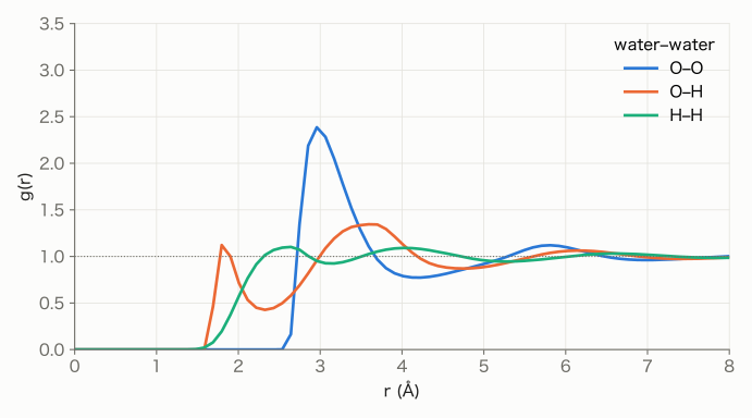
• O–O: a high peak at 2.96 Å (\(g\approx2.4\)), the first hydration shell of water molecules.
• O–H (between different molecules): the small peak around 1.8 Å corresponds to the hydrogen bond.
• At large distances all curves approach 1, a uniform liquid.

Hydration of ions

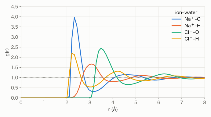
• Na⁺: the Na⁺–O peak (2.32 Å, \(g\approx4.0\)) lies inside the Na⁺–H peak (3.06 Å). Water oxygens point toward the cation.
• Cl⁻: the Cl⁻–H peak (2.22 Å) lies inside the Cl⁻–O peak (3.49 Å). Water hydrogens point toward the anion.

The distribution functions show how the orientation of water molecules flips with the sign of the ionic charge.

Chemical potential of solvation

After 1D-RISM, the chemical potential of solvation (excess chemical potential) of each solvent species in the solution is printed.

     Chemical potential of solvation

     H2O        H2O        Closure     -0.153796E+01 kcal/mol
                ...
                Total      Closure     -0.229340E+01 kcal/mol
                           GaussFluct  -0.583926E+01 kcal/mol

     Na+        H2O        Closure     -0.446607E+02 kcal/mol
                Na+        Closure      0.175759E+06 kcal/mol
                Cl-        Closure     -0.175796E+06 kcal/mol
                Total      Closure     -0.820464E+02 kcal/mol

Species	Closure (kcal/mol)	GaussFluct (kcal/mol)
H2O	−2.29	−5.84
Na+	−82.0	−84.3
Cl−	−76.4	−79.2

• Closure is evaluated with the expression corresponding to the closure (here KH), and GaussFluct with the Gaussian fluctuation (GF) approximation.
• The ion–ion components (Na⁺–Na⁺, Na⁺–Cl⁻, …) are individually large but cancel each other; only the Total is meaningful.

The structure of the solution obtained here by 1D-RISM is the basis of the following 3D-RISM and ESM-RISM calculations.