ESM Tutorial

This tutorial runs the ESM example distributed with Quantum ESPRESSO (PW/examples/ESM_example) and plots the planar-averaged electron density and potential it writes out, to show what the ESM method changes. For the theory, see the ESM method.

Setup

The ESM method is switched on by two keywords in the &system namelist.

 &system
    ...
    assume_isolated = 'esm'
    esm_bc = 'bc1'      ! 'pbc', 'bc1', 'bc2', 'bc3'
 /

esm_bc selects the media placed on both outer sides of the slab (or molecule).

esm_bc	Left (\(z<0\))	Right (\(z>0\))	Typical use
pbc	periodic boundary condition (ESM off)	same	reference
bc1	vacuum	vacuum	isolated slabs and molecules
bc2	metal	metal	systems under an applied field (capacitor)
bc3	vacuum	metal	charged electrode surfaces (with a counter electrode)

Run the example as follows. Each calculation finishes in a few seconds.

cd q-e/PW/examples/ESM_example
./run_example_ESM

The total energies and Fermi energies shown here agree to all printed digits with the reference outputs distributed with the example (reference/). The H₂O bc2 and bc3 runs are additional calculations, made by changing only esm_bc in H2O_bc1.in.

The output file *.esm1

With ESM (including esm_bc='pbc'), the code writes the electron density and potentials averaged over the plane (\(xy\)) to prefix.esm1.

#z (A)  Tot chg (e/A)  Avg v_hartree (eV)  Avg v_local (eV)  Avg v_hart+v_loc (eV)
 -6.00           0.0000048        -198.6208627       198.6194404        -0.0014223

Column	Content
1	\(z\) (Å)
2	planar-averaged electron density (e/Å; electrons counted positive, integrates to the number of electrons)
3	Hartree potential (eV)
4	local pseudopotential (eV)
5	sum of columns 3 and 4 (eV)

The figures below plot column 5, the electrostatic potential energy felt by an electron.

1. A molecule with a dipole: H₂O

An H₂O molecule with its dipole along \(z\) (cell 10.58 × 10.58 × 12.70 Å, \(\Gamma\) point) is computed with the four boundary conditions.

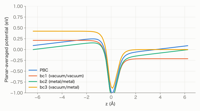
• PBC: the potential is tilted in the vacuum region. Periodicity forces the potential to take the same value at both cell ends, so the periodic array of dipoles creates an artificial electric field across the cell.
• bc1 (vacuum/vacuum): the vacuum regions on both sides are flat, and they differ by 0.424 eV. This is the step in the vacuum level caused by the molecular dipole, the correct picture of an isolated molecule.
• bc2 (metal/metal): the potential is fixed to zero at the metals on both ends. The image charges induced in the metals counteract the dipole, so the vacuum regions are tilted.
• bc3 (vacuum/metal): the potential is fixed to zero at the metal on the right, and the vacuum on the left is flat.

The total energy changes slightly. The difference from PBC comes from the interaction between periodic dipoles (PBC) or with the image charges (bc2).

esm_bc	Total energy (Ry)	Difference from PBC (meV)
pbc	−34.43089505	0
bc1	−34.43056646	+4.47
bc2	−34.43090315	−0.11
bc3	−34.43057080	+4.41

2. Fermi energy of a metal slab: Al(001)

For a neutral one-layer Al(001) slab (4 atoms, \(6\times6\times1\) \(k\)-points), the Fermi energies are:

esm_bc	Fermi energy (eV)
pbc	−2.0409
bc1	−4.2462
bc2	−4.2503
bc3	−4.2474

With periodic boundary conditions the average potential in the cell is set to zero, so the energy reference has no physical meaning. With ESM the potential vanishes in the vacuum (or metal) at infinity, so the Fermi energy is measured from the vacuum level and equals minus the work function (about 4.25 eV). These values belong to the one-layer, low-cutoff model of the example.

3. A charged electrode: bc3 and tot_charge

With bc3, give the system an excess charge (tot_charge = -0.02: 0.02 electrons added; +0.02: 0.02 electrons removed). The compensating charge is carried by the ESM metal, so no uniform background charge is needed.

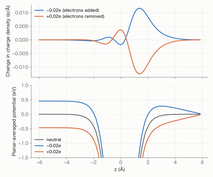
• Change in electron density (top): the excess charge collects at the surface facing the metal (right). The surface facing the vacuum on the left hardly changes.
• Potential (bottom): an electric field appears only between the slab and the metal (the slope on the right), while the vacuum on the left stays flat and shifts as a whole. The model is an electrode surface facing a counter electrode, that is, one side of a capacitor.

Relative to the neutral slab (−4.25 eV), the Fermi energy becomes −3.80 eV for −0.02e and −4.71 eV for +0.02e, a change of 0.458 V on average. Per area (32.8 Ų) this is a capacitance of about 2.1 μF/cm², which for a vacuum parallel-plate capacitor \(C=\varepsilon_0/d\) corresponds to \(d\approx4.2\) Å, roughly the distance from the slab surface to the metal.

4. Applying a field: bc2 and esm_efield

With bc2 and esm_efield = 0.00192148511256006 (Ry/bohr, about 0.049 V/Å), a uniform field is applied between the metals on both sides.

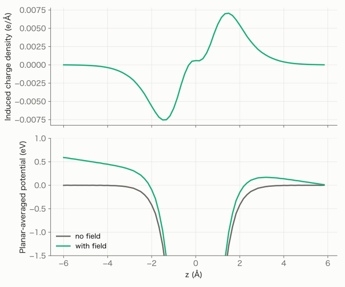
• Induced charge (top): electrons move toward the right surface and leave the left surface. The slab polarizes and screens the field from its interior.
• Potential (bottom): both vacuum regions are tilted by the applied field. The potential difference between the two metals corresponds to the field times the cell length (0.049 V/Å × 12 Å ≈ 0.59 V).

5. Keeping the electrode potential constant: FCP and GC-SCF

So far we have specified the charge (tot_charge). In real electrochemistry, the electrode potential is specified and the charge follows from it. The constant-μ method does this: given a target Fermi energy \(\mu\), it adjusts the charge of the system automatically. The examples (run_example_FCP, run_example_GCSCF) target potentials ±0.5 V away from the Fermi energy of the neutral slab (the potential of zero charge, pzc). Since the electrode potential \(U\) and the Fermi energy are related by \(U-U_\mathrm{pzc}=-(\mu-\mu_\mathrm{pzc})/e\), a target of +0.5 V means \(\mu=\mu_\mathrm{pzc}-0.5\) eV.

Quantum ESPRESSO offers two methods.

! FCP: the charge is relaxed in an outer loop around the SCF
 &control
    calculation = 'relax'
    lfcp = .TRUE.
 /
 &fcp
    fcp_mu = -4.7490          ! target Fermi energy (eV)
    fcp_dynamics = 'bfgs'
    fcp_conv_thr = 1.d-2      ! eV
    freeze_all_atoms = .TRUE. ! move only the charge
 /

! GC-SCF: the charge is adjusted inside the SCF loop
 &control
    calculation = 'scf'
 /
 &system
    lgcscf = .TRUE.
    gcscf_mu = -4.7490        ! target Fermi energy (eV)
    gcscf_conv_thr = 1.d-2    ! eV
 /

• FCP (fictitious charge particle): the charge is treated as the coordinate of a fictitious particle, and the difference between the Fermi energy and its target acts as a "force" that moves the charge outside the SCF loop. The SCF is solved again after every change of charge.
• GC-SCF (grand-canonical SCF): the charge is updated together with the electron density inside the SCF iterations, so the charge and the Fermi energy converge in a single SCF.

For bc3 with targets of +0.5 V and −0.5 V, the figure compares how the Fermi energy and the charge evolve against the cumulative number of SCF iterations.

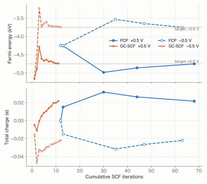
FCP (blue) updates the charge each time an SCF has converged, so about 10–20 SCF iterations lie between consecutive points. With GC-SCF (orange) the charge moves toward its target within one SCF and converges in about 10 iterations. The final charges of the two methods are nearly the same.

Boundary condition	Target	FCP: SCF runs	FCP: total iterations	FCP: charge (e)	GC-SCF: iterations	GC-SCF: charge (e)
bc3	+0.5 V	5	68	+0.0217	11	+0.0218
bc3	−0.5 V	5	63	−0.0220	12	−0.0219
bc2	+0.5 V	3	25	+0.0437	10	+0.0438
bc2	−0.5 V	5	57	−0.0437	12	−0.0436

The results show the following.

• With bc3, about 0.0218 e flows in or out per 0.5 V. This agrees with the capacitance estimated from the charge in Section 3 (0.458 V for 0.02 e).
• With bc2, about twice as much charge flows. Both faces of the slab face a metal, so two capacitors act in parallel.
• The two methods spend their iterations differently. GC-SCF reaches the target potential in a single SCF and is therefore efficient, but because the electron density and the charge converge together, that single SCF tends to need more iterations (the example uses a smaller density mixing, mixing_beta = 0.1; since the system is small, it still took only 11–12 iterations, about the same as the neutral SCF with 12). In FCP, each SCF is an ordinary SCF at a fixed number of electrons, so each one tends to be short, but repeating it several times makes the total number of iterations larger.

From these characteristics, GC-SCF is the better choice for adjusting the Fermi energy of a fixed structure. FCP, which treats the charge with an equation of motion, is the better choice when combined with molecular dynamics to move atoms at a constant potential: in MD the charge and density of the previous step are good initial guesses, so each fixed-electron-number SCF stays short (see the Constant-μ method).

Summary

What you want	Boundary condition	What ESM gives
systems with a dipole, asymmetric slabs	bc1	an isolated system without an artificial field, and the vacuum-level step
work functions and absolute energy levels	bc1–bc3	Fermi energies referenced to the vacuum (or metal)
charged electrode surfaces	bc3 + tot_charge	charge distribution and capacitance including the counter electrode
systems under an applied field	bc2 + esm_efield	polarization and screening
electrodes at a given potential	bc2/bc3 + FCP / GC-SCF	charge and capacitance as functions of potential